Application of Bayesian predictive probability for interim futility analysis in single-arm phase II trial
Introduction
Recent modern biomedical research has generated golden opportunities of exploring various potential experimental drug agents and/or combinations of existing drugs to fight against cancer, such as nivolumab (1-3), ipilimumab (4,5), and pembrolizumab (6,7) in immunotherapy, ceritinib (8-10) and crizotinib (11-13) in targeted therapy, and the combinations with other drugs (4,5,14-19). The drug efficacy is often evaluated in phase II clinical trials. Many phase II clinical trials utilize Simon two-stage design (20) to early terminate ineffective drugs and identify effective drugs to warrant a phase III trial (14-19,21-23). The method deterministically defines the interim and final analyses and sample sizes for given type I and II errors. While it is popular, some studies may require pre-determined sample sizes and therefore could limit Simon two-stage design’s application. This also presents a challenge of how to design a statistically justified interim analysis under the constraints of pre-defined sample sizes. The issue could be easily addressed by the Bayesian approach.
Many Bayesian approaches have been proposed for phase II single arm design either by posterior probability, predictive probability, or even incorporating with frequentist approach. Most of them are limited to a Simon like two-stage, such as Tan and Machin (24) using posterior distribution for decision, Sambucini (25,26) and Liu et al. (27) using Bayesian predictive strategies, and Wang et al. (28) using a hybrid of frequentist and Bayesian error rates. For continuously monitoring a schema Thall and Simon (29) used posterior probability to define stopping rules while Lee and Liu (30) and Saville et al. (31) used predictive probability to construct the boundary.
In this study, we utilize the Bayesian posterior probability and predictive probability by Lee and Liu (30) to construct a statistical plan in clinical trial design for a binary endpoint. This approach has several useful features, such as flexible options to manage the futility assessment at the interim analysis, as well as integration of both the posterior probability and the predictive probability to define the stopping rule for futility. Here we present the developed R package for this Bayesian design and share our experiences of the real application, so the oncology research community can easily adapt the design into their clinical trial protocols.
Methods
Concept
The Bayesian posterior probability and predictive probability (30) uses a few simple but powerful concepts to construct the design. The posterior probability is defined as a probability that the targeted treatment’s response rate is greater than the one in the null hypothesis. A large value indicates a high degree of promising treatment results. Thus, it can be used to determine efficacy. The predictive probability is likelihood to reach treatment efficacy at the end of the study given the number of responders observed at the current status. When it is close to 0, the chance to claim success becomes unlikely. Therefore, the predictive probability is a useful tool to outline the stopping rule in interim analysis to reflect the chance of early termination. Specifically, given the null hypothesis, sample size, and prior information, the design first utilizes the posterior probability to decide treatment efficacy. If the probability is higher than a threshold, it indicates effectiveness of the treatment. As a result, it defines the minimum number of responders needed for efficacy for a given total sample size. Then the predictive probability is applied at each interim analysis to construct the stopping rule with a cutoff. If the predictive probability is below the cutoff, it indicates the treatment is futile and the action of early termination should be considered.
Algorithm
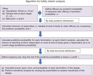
The concept above leads to the following algorithm (Figure 1 summarizes the algorithm).
Select beta prior for the treatment response data
Information about response data of the experimental treatment helps determine the beta prior distribution, beta(a,b), for the response rate where a represents the degree of response (e.g., number of responders) while b indicates magnitude of non-response (e.g., number of non-responders). The mean response rate is a/(a+b) with a>b for tendency of more drug-sensitive, a<b for more drug-resistant, and a=b for undetermined. In addition, when a+b becomes large, the belief of prior information gets strong and likely dominates the result. While many experimental treatments are usually the first study, some of them are a combination of standard treatment with new drug or modification of standard treatment. Thus, utilization of historical data could help better shape prior distribution within the Bayesian framework. Often prior information provided by a physician is not the values of a and b, but a response rate estimate. Conversion to the two parameters (a and b) can be done by a formula with a hypothesized standard deviation (SD) of response rate:
where p is the mean response rate.
Setup hypothesis and sample size
We consider a null hypothesis of treatment with a response rate ≤ p0 and an alternative hypothesis of the response rate ≥ p1. In addition, sample size at each stage is allocated with ni denoting the sample size of patients in the ith interim analysis and n as the total sample size.
Define treatment efficacy by posterior probability and determine minimum number of total responders
We claim that the treatment is promising (efficacy) if the posterior probability is higher than a threshold, δ, for 0< δ <1 [i.e., prob(response rate > p0 |data)> δ]. Thus, with a total of n patients, the minimum of responders, k, to claim efficacy can be determined by the following mathematical form with a posterior beta(a+k,b+n-k) distribution for the response rate:
where B(a,b) is the beta function. Calculation of k will be done by the equation:
Calculate the predictive probability for early termination
Given the number of responders, s, in the first n1 patients, we calculate the predictive probability of ≥ k-s responders in future n* (where n* =n-n1) patients, i.e.,
The beauty of this predictive probability is that the formula follows a beta binominal distribution, BetaBinom(n*,a-s,b+(n1-s)). Thus, we are able to analytically calculate the predictive probability for the number of responders among the remaining n* patients given the currently updated response rate, which has a beta distribution, beta(a+s,b+n1-s). The predictive probability is also calculated similarly for each of the remaining interim analyses to evaluate the chance of k-s or more responders in the remaining n* patients given s responders in the current stage of interim analysis. That is, for the lth stage with the cumulative sample size,
the predictive probability becomes a beta binominal distribution,
with the formula:
where , the future sample size.
Set up a stopping rule
The predictive probability is a useful tool as a stopping rule. It can be used to end a trial early for futility purpose when the probability is low. By setting a cutoff of the predictive probability, γ, to indicate unfavorable likelihood for success, the number of responders, , for the stopping boundary at lth stage can be easily calculated by the beta-binomial distribution. That is,
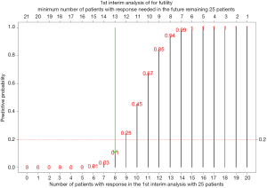
For example of a two-stage design with p0=0.3, , n2=25 (n*=25), a=1, b1=1, and δ=0.95 (lead to k=21), if the number of responders in the 1st stage is 0 (s=0), the predictive probability to have 21 responders in the 2nd stage (k-s=21) is close to 0 (<0.0001). For s=1-7, the predictive probability to have 20-14 responders in the 2nd stage is <0.05. When s=8 and 9, the predictive probability to have 13 and 12 responders in the 2nd stage is 0.11 and 0.25, respectively. Thus, for a cutoff of 0.2 (γ=0.2), the stopping boundary is 8 responders in the 1st stage ().
Another function is to stop the trial for efficacy if the predictive probability is very high. However, due to the nature of small sample size in early phase II trial, it is less feasible.
Evaluate performance of the design
The stopping rule characterizes the study design and provides the stopping boundary at each stage, for stage l. We further decompose the boundary, where ki is the additional number of responders needed in stage I. With the decomposition, sample size of each stage, and response rate of null and alternative hypotheses (p0 and p1), the analytical form can be derived for probability of early termination (PET) of the trial, type I error, and power to assess performance of the design.
- PET: It is a probability to stop the trial before going to the final stage. For a two-stage design, it is the probability of trial termination at the 1st stage, i.e.,
- by binominal distribution. For a 3-stage design, it becomes
- For a m-stage design (m >3),
- Type I error: It is a probability of accepting treatment efficacy when the true response rate is p0. The probability is 1-the sum of PET(p0) and the probability of failure to reach the efficacy at the final stage. That is,
15]
- For a two-stage design,
- Power: It is defined as the probability of claiming efficacy when the true response rate is p1. That is,
Perform sensitivity analysis
Sensitivity analysis will be conducted to evaluate performance of the design in terms of PET, type I error, and power. Four parameters associated with the performance are explored: (I) γ, cutoff of the predictive probability. The cutoff will form a stopping boundary, and therefore affect PET, type I error, and power, (II) δ, threshold for posterior probability of response rate. It determines minimum number of total responders to claim efficacy and decides power and type I error, (III) sample size, and (IV) prior information of the response rate. Both sample size and prior information also control the minimum number of total responders for efficacy and stopping boundary for futility. The impact of each parameter on performance will be examined when other parameters are fixed. Sensitivity analysis provides opportunity to evaluate robustness of the design and tune up the design by changing key parameters.
Results
Demonstration
We use three cases to illustrate utility of the approach: two-, three-, and multi-stage (details are in the Supplementary materials for demonstration). The following setting is used for demonstration: the response rate is 30% in the null hypothesis (unfavorable response rate) and 50% in the alternative hypothesis (the minimum favorable response rate). The pre-defined sample size is 50 subjects in total. A non-informative beta prior, beta(1,1), is used to calculate the response rate. The treatment is considered promising if the posterior probability is higher than 0.95 [i.e., prob(response rate>30% |data)>0.95]. Thus, with a total of 50 patients and by solving the equation,
we will need at least 21 responders (i.e., k=21) to claim efficacy by the beta posterior probability.
Two-stage case
One interim analysis is considered at the first 25 subjects (equal split). That is, the 1st stage enrolls 25 patients and the final stage has an additional 25 patients if the trial passes the 1st stage (Table 1).
Table 1
| Design | Stage of interim analysis | Sample size at each stage | Sample size up to the current stage | Stopping boundary | Performance |
|---|---|---|---|---|---|
| Two-stage | 1 | 25 | 25 | 8 | 88% power; 4% type I error; 68% probability of early termination |
| Final | 25 | 50 | 20 | ||
| Three-stage | 1 | 15 | 15 | 4 | 85% power; 4% type I error; 77% probability of early termination |
| 2 | 15 | 30 | 10 | ||
| Final | 20 | 50 | 20 | ||
| Multi-stage | 1 | 10 | 10 | 2 | 83% power; 4% type I error; 91% probability of early termination |
| 2 | 10 | 20 | 6 | ||
| 3 | 10 | 30 | 10 | ||
| 4 | 10 | 40 | 15 | ||
| Final | 10 | 50 | 20 |
Given the number of responders, s, in the first 25 patients for the 1st stage, we calculate predictive probability of 21-s or more responders in the remaining 25 patients, i.e.,
Calculation of the predictive probability is based on beta binominal distribution for the number of responders in the remaining 25 patients given a beta distribution for the response rate, beta(1+s,1+25-s). For example, if there are 8 patients with response in the first 25 patients, the predictive probability of 13 or more patients with response in the future remaining 25 patients would be
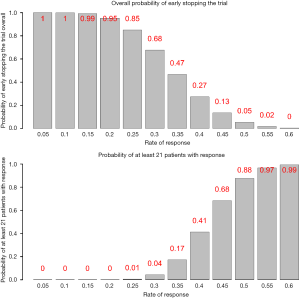
Figure 2 lists the predictive probability for all scenarios of number of responders in the first 25 patients (interim analysis) and number of responders needed in the remaining 25 patients to have at least a total of 21 responders. With γ=20%, the stopping rule (Table 1) is if there are 8 responders or less for the first 25 patients in the interim analysis, we consider the treatment as ineffective and the trial will be stopped. Performance of this stopping rule (Figure 3) shows that if the true response rate is 30%, the chance to reach a total of 21 responders at end of the study is 0.04 (type I error) with 68% PET. On the other hand, if the true response rate is 50% (20% higher than the 30% response rate), the power is 88% to reach a total of at least 21 responders at end of the study.
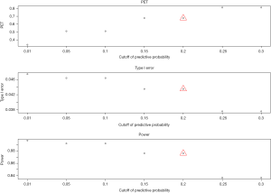
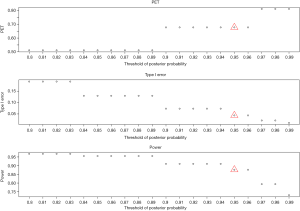
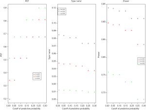
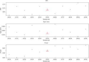
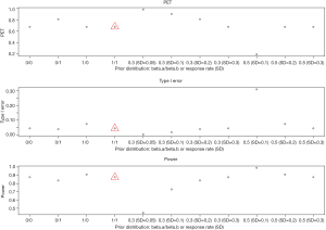
Sensitivity analysis shows that when the cutoff of the predictive probability for the stopping rule is 0.01–0.3, the range is 0.34–0.81 for PET, 0.04–0.05 for type I error, and 0.84–0.9 for power. When the threshold for posterior probability to define efficacy is 0.8–0.99, the range is 0.51–0.81 for PET, 0.01–0.19 for type I error, and 0.73–0.97 for power. When the sample size of each stage is in the magnitude from decrease by −5 to increase by 5, the range is 0.61–0.77 for PET, 0.04–0.07 for type I error, and 0.82–0.92 for power. When the beta prior varies from non-informative prior to the one with a response rate at the null or alternative hypothesis and a series of standard deviation (SD), the range is 0.19–0.98 for PET, 0–0.31 for type I error, and 0.45–0.99 for power.
Three-stage case
Two interim analyses are planned with 15, 15, and 20 patients in the 1st, 2nd, and final stage (Table 1). Given the same 20% cutoff of the predictive probability, the stopping rule will be: the trial will be stopped if there are 4 and 10 or less responders in the 1st and 2nd interim analysis, respectively (Table 1). The design has 85% power, 4% type I error, and 77% of early termination. Details including sensitivity analysis are in Supplementary materials for demonstration.
Multiple-stage case
The design includes 4 interim analyses with 10 patients in each stage (Table 1). With a 20% cutoff for the predictive probability, the stopping rule (Table 1) will be: the trial will be stopped if there are 2, 6, 10, and 15 or less responders in the 1st to 4th interim analysis, respectively. The design shows 83% power, 4% type I error, and 91% of early termination. Details including sensitivity analysis are in Supplementary Materials for Demonstration.
The three different stage cases show a similar statistical power ranging 83–88% and a 4% type I error. However, the PET increases as the frequency of interim analysis increases (68% to 91%).
Detailed sensitivity analysis for the two-stage case
- Cutoff of the predictive probability, γ: as the cutoff of the predictive probability decreases from 0.3 to 0.01 (Figure 4), power increases (90% down to 84%), but PET decreases (81% down to 34%) and type I error increases (4% up to 5%). The impact is substantial on PET, moderate on power, and little on type I error.
- Threshold of the posterior probability, δ: when the threshold for posterior probability increases from 0.8 to 0.99 (Figure 5), power decreases from 97% to 73%. In contrast, PET increases from 51% up to 81% and type I error decreases from 0.19 down to 0.01. All the three metrics (PET, type I error, and power) are largely impacted by the threshold of the posterior probability.
- Joint effect of γ and δ: three thresholds of the posterior probability (δ=0.90, 0.95, and 0.99) are evaluated with the cutoff of the predictive probability from γ=0.01 to 0.3 to examine the joint effect in Figure 6. PET increases as both γ and δ increase. For δ=0.9, PET has 48% difference (from 19% to 68%) when γ increases from 0.01 to 0.3. However, as δ increases to 0.99, the change of PET decreases (39% difference) for the same range of γ (0.01 to 0.3). For type I error, when δ=0.9, it ranges 7% to 8% (~1% difference) for a γ of 0.01 to 0.3. As δ increases to 0.99, the difference of type I error becomes negligible (<0.005). In evaluation of power, δ of 0.9 gives a range of power from 91% to 94% (3% difference) for a γ of 0.01 to 0.3. As δ increases to 0.99, power decreases to 68–76% (8% difference) for the same range of γ. The results indicate the joint effect has a large impact on PET, mild effect in power, and little influence in type I error.
- Sample size: change of sample size does not always increase power and PET and reduce type I error (Figure 7). It does not follow a monotonic form, but a quasi-systematic up- and down-pattern. For example, when sample size increases from 21 to 23 in each stage, it decreases PET (from 0.72 to 0.62) and increases power (from 82% to 89%). The type I error is 5%, 4%, and then 6% (down then up). The similar pattern occurs for a sample size of 24 to 27 in each stage. The cycle restarts for a sample size of 28–29. While the irregular pattern presents some challenges in determining a right sample size, the effect is mild on the three metrics. This may be due to the discreteness of the beta-binominal distribution.
- Beta prior: non-informative priors have mild impact on power (84–91%) and type I error (4–7%), but a large change on PET (68–81%) as shown in Figure 8. The prior based on a response rate at the null or alternative hypothesis also gives a similar effect when the SD is large (e.g., ≥0.3). When SD is small (e.g., ≤0.1), the sum of two beta parameter values (a and b) significantly increases and therefore dominates the results. For example, when the prior is based on the response rate at null hypothesis (30%) with SD =0.05, the values of two beta parameters increase: a =24.9 and b =58.1. It will need a total of at least 23 responders (out of 50 patients) to claim efficacy. The trial will be stopped early if there are 12 responders or less in the 1st stage. As a result, the trial design could be easily terminated in the 1st stage with a 98% PET, with a low power of 45%. On the other hand, for a prior using the response rate at alternative hypothesis (50%) with SD =0.1 (a = b =12), a total of at least 16 responders is needed to claim efficacy. The design has a low chance to terminate the trial (PET =19%) because it only requires 5 responders or less in the 1st stage to stop the trial. While the design has a high power of 99%, it also has a high type I error, 31%.
Development of a statistical tool, BayesianPredictiveFutility R package
A R package, ‘BayesianPredictiveFutility’, with associated graphical interface (R Shiny App) is developed for easy utilization of the trial design (source code at https://github.com/dungtsa/BayesianPredictiveFutility). The unique feature of the statistical tool is to generate a professional statistical plan for biostatisticians and clinicians to easily incorporate into their clinical trial protocols. The statistical plan presents the methodology in a readable language fashion while preserving rigorous statistical arguments.
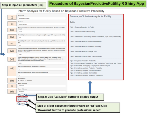
Once the R package is installed and loaded, the command line ‘Bayesian_Predictive_App()’ in R console will open a R Shiny app tool in a web browser for users to input the parameters as shown in Figure 9 with graphical illustration.
The tool requires a set of parameters for input:
- Project title: title of the proposed clinical protocol.
- Authors: list of primary and co-investigators.
- Sample size: sample size for each interim analysis with comma delimited for separation (e.g., 25, 25 for 1st and 2nd stage).
- Probability under the null hypothesis (p0) (e.g., p0=30% response rate at H0).
- Probability under the alternative hypothesis (p1) (e.g., p1=50% response rate at H1).
- Threshold of posterior probability to define treatment efficacy: the range is 0–100% but a suggested value is 80–99%. A higher threshold requires a larger number of responders to claim efficacy and leads to a lower power.
- Cutoff of predictive probability to define stopping rule: The range is 0–100%, but a suggested value is 0.01–0.3. A higher threshold requires a larger number of responders to advance to the next stage and leads to terminate the trial early.
- beta a and b parameters: Both parameters represent the degree of response and nonresponse, respectively, with a>b for tendency of more drug-sensitive, a<b for more drug-resistant, and a=b for undetermined. In addition, when a+b becomes large, the belief of prior information gets strong and likely dominates the result.
- Analysis type: two options are available: analytical analysis and simulation. Analytic analysis is recommended for computation efficiency. Simulation may be feasible when many interim analyses are required.
- Name of outcome: it could be ‘response’ if response rate is the primary endpoint.
- Name of the arm: the name of the treatment arm.
With the input of all parameters, clicking the ‘Calculation’ button will generate a comprehensive report, including a summary, details of study design, a series of tables and figures from stopping boundary for futility, Bayesian predictive probability, performance (PET, type I error, and power), PET at each interim analysis, sensitivity analysis for predictive probability, posterior probability, sample size, and beta prior distribution (labelled as Tables 1-7 and Figures 1-7, respectively, in the report). The output formats (Word or PDF) are available to communicate with physicians or to be incorporated in the trial protocol.
Table 2
| Method | k1 | n1 | k−1 | n | Type I error | Power | PET |
|---|---|---|---|---|---|---|---|
| Immunotherapy naïve cohort: 30% versus 50% response rate | |||||||
| Bayesian predictive probability | 6 | 20 | 16 | 40 | 6% | 85% | 61% |
| Minimax | 6 | 19 | 16 | 39 | 5% | 80% | 67% |
| Optimum | 5 | 15 | 18 | 46 | 5% | 80% | 72% |
| Immunotherapy treated previously cohort: 7% versus 20% response rate | |||||||
| Bayesian predictive probability | 1 | 20 | 5 | 40 | 5% | 82% | 59% |
| Minimax | 1 | 21 | 5 | 39 | 5% | 80% | 56% |
| Optimum | 1 | 16 | 6 | 50 | 5% | 80% | 69% |
| Ceritinib and Docetaxel cohort: 12% versus 32% response rate | |||||||
| Bayesian predictive probability | 2 | 15 | 6 | 30 | 5% | 84% | 73% |
| Minimax | 2 | 17 | 6 | 27 | 4% | 80% | 67% |
| Optimum | 2 | 13 | 6 | 31 | 5% | 80% | 80% |
Application of the R package
Application of two clinical trials in lung cancer is used to demonstrate its usefulness: one single arm phase II trial and one phase IB trial (NCT03377023 and NCT03611738 in ClinicalTrials.gov). A non-informative beta prior, beta(1,1), is used for the Bayesian posterior probability and predictive probability. Two-stage design is employed for both trials (detailed statistical justification is in the Supplementary Materials for Application).
The phase II trial is an immunotherapy study to evaluate a combined treatment of nivolumab, ipilimumab, and nintedanib in advanced non-small cell lung cancer (NSCLC). Two cohorts are studied: immunotherapy naïve and immunotherapy treated previously. For each cohort, the two-stage design includes 20 patients in each stage. We consider that the treatment is promising if the posterior probability of response rate greater than a least favorable response rate, p0, is higher than 0.95 [i.e., prob(response rate>p0 |data)>0.95]. The p0 is 30% and 7% for the immunotherapy naïve cohort and the immunotherapy treated previously cohort, respectively. The alternative hypothesis is 20% and 13% improvement of the response rate (i.e., p1=50% and 20%), accordingly. With a 20% cutoff of the predictive probability, for the immunotherapy naïve cohort, the stopping rule is 6 or less responders in the 1st stage. If a total of responders are 17 or more (out of a total of 40 patients), the treatment is considered promising and deserves further examination in future randomized phase II or III trials. The operation characteristics has an 85% power, a 6% type I error, and a 61% PET. For the immunotherapy treated previously cohort, the stopping rule is 1 or no responder in the 1st stage. The treatment is considered promising if a total of responders are 6 or more. The design has an 82% power, a 5% type I error, and a 59% PET.
The phase IB trial is to evaluate efficacy of combination of two drugs, Ceritinib and Docetaxel, in patients with locally advanced or metastatic NSCLC after failure of prior platinum therapy. A futility analysis is included in the interim analysis to stop the trial earlier if the treatment does not work well. A pre-defined sample size is a total of 30 patients with one interim analysis after 15 patients have response data. The hypothesis is a response rate of 12% as a least favorable response rate (null hypothesis) and 32% as the minimum encouraging response rate (alternative hypothesis). The treatment is considered promising if the posterior probability of the response rate greater than 12% is higher than 0.95 [i.e., prob(response rate>12% |data)>0.95]. The statistical design is based on a cutoff of 20% for the predictive probability. The stopping rule is 2 or less responders in the interim analysis. It requires a minimum number of 7 responders at end of the study to warrant further randomized trials. The design has an 84% statistical power, a 5% type I error, and a 73% PET.
Comparison to Simon two-stage design
Simon two-stage design (20) has two types: optimal and minimax design. The optimal design aims to minimize the expected sample size under the null hypothesis while the minimax design targets the smallest maximum sample size. The optimal design often has a larger sample size compared to the minimax design. The optimal design conducts the interim analysis usually earlier with less than 50% of the total sample size. In contrast, the minimax design tends to implement the interim analysis at late stage using more than 50% of the total sample size.
For the immunotherapy naïve cohort, the Simon minimax design yields a total of 39 subjects with 19 in the 1st stage and a 67% PET (Table 2). For the optimum design, the sample size increases to 46 subjects, with 15 subjects in the 1st stage and 72% PET. The Simon minimax design is close to the design by Bayesian predictive probability in terms of sample sizes and stopping rule. The Bayesian predictive probability approach gives a higher statistical power (85% versus 80%), but a lower PET (61% versus 67%). The optimum design requires a 15% increase of sample size (46 versus 40). Both Simon designs are unable to give a balanced sample size at each stage. The immunotherapy treated previously cohort also gives a similar comparison result (Table 2). For the Ceritinib and Docetaxel cohort in the phase IB trial, the Simon minimax design gives a smaller total sample size (n=27), but it requires the interim analysis conducted after 63% patients with response data, rather than earlier (Table 2). Also, the statistical power and PET are smaller compared to the Bayesian predictive probability approach (power: 80% versus 84%; PET: 67% versus 73%). The optimal design is similar to the Bayesian approach.
Discussion
In general, the Simon two-stage design is widely used in the single arm phase II clinical trial. Here, we apply an alternative approach, Bayesian strategy (30), for futility analysis. It employs the predictive probability, to construct stopping rule by evaluating the chance of future success. It allows flexibility of sample size in each interim analysis. It gives freedom for a desirable PET, as well as an interpretable stopping rule for interim futility analysis. The statistical R package (‘BayesianPredictiveFutility’), we developed provides great opportunity to broaden the application in clinical trial. We have applied this statistical tool for the Bayesian approach in two ongoing clinical trials, one for immunotherapy and one for targeted therapy, to demonstrate its usefulness as shown in the Section of Application of the R Package.
For clinical investigators, the Bayesian approach holds unique strengths over the Simon two-stage design. One key feature is the freedom to determine the number of patients in the interim analysis. Sometimes the investigator may request a customized sample size schema (e.g., a balanced sample size across the stages or a pre-determined sample size) for futility analysis in single arm phase II trial. Examples in the Section of Application of the R Package are the cases with equal sample sizes in the 1st and 2nd stages. The Simon two-stage design gives an unbalanced design with different sample sizes either by minimax or optimal criteria. The Bayesian approach can address this issue with an interpretable futility analysis plan and comparable power and type I error. Moreover, with sensitivity analysis, it allows investigators to select a desirable PET to better determine an appropriate stopping rule for trials (Sensitivity Analysis in Result Section). The other uniqueness is its adaption of the predictive probability to evaluate the future success at interim stage. The low chance of future success could become an ethical reason to stop the trial. In contrast, some approaches, such as classic group sequential trials, use interim P values for the stopping rule which may allow trials with very low probabilities of success to continue (31).
With the goal to make this Bayesian design more accessible, the R package, ‘BayesianPredictiveFutility’, provides a graphical user interface for easy implementation. Our suggested strategy is to start with two key parameters: the threshold of the posterior probability, δ, and the cutoff for the predictive probability, γ, because δ dominates power and type I error and γ controls the PET (Sensitivity Analysis in Result Section). Once all parameters are entered, the tool will generate a professional report to describe what the study design is (e.g., when to stop the trial), how the design is derived (e.g., how the stopping rule is formularized), and how robustness the design is (e.g., sensitivity analysis by varying key parameters), with a series of tables and plots to support the design. The Word or PDF output format is another plus to give clinicians to easily incorporate the design report into clinical trial protocol.
In summary, the Bayesian predictive probability presents a high degree of flexibility for futility assessment at the interim analyses in single arm phase II clinical trials. The statistical tool brings potential benefit for easy implementation in trial design.
Supplementary
Supplementary materials for demonstration
- Two-stage: calculation of predictive probability, development of stopping boundary, and sensitivity analysis;
- Three-stage: calculation of predictive probability, development of stopping boundary, and sensitivity analysis;
- Multi-stage: calculation of predictive probability, development of stopping boundary, and sensitivity analysis.
Supplementary materials for application
- Cohort 1 (immunotherapy naïve): calculation of predictive probability, development of stopping boundary, and sensitivity analysis;
- Cohort 1 (immuno therapy pretreated): calculation of predictive probability, development of stopping boundary, and sensitivity analysis;
- Cohort 2 (targeted therapy): calculation of predictive probability, development of stopping boundary, and sensitivity analysis.
Supplementary
Acknowledgments
We thank Mrs. Paula D. Price for editorial assistance.
Funding: Support for this study included departmental funds from
Footnote
Provenance and Peer Review: This article was commissioned by the Guest Editors (Hui-Yi Lin, Tung-Sung Tseng) for the series “Population Science in Cancer” published in Translational Cancer Research. The article has undergone external peer review.
Conflicts of Interest: All authors have completed the ICMJE uniform disclosure form (available at http://dx.doi.org/10.21037/tcr.2019.05.17). The series “Population Science in Cancer” was commissioned by the editorial office without any funding or sponsorship. The authors have no other conflicts of interest to declare.
Ethical Statement: The authors are accountable for all aspects of the work in ensuring that questions related to the accuracy or integrity of any part of the work are appropriately investigated and resolved.
Open Access Statement: This is an Open Access article distributed in accordance with the Creative Commons Attribution-NonCommercial-NoDerivs 4.0 International License (CC BY-NC-ND 4.0), which permits the non-commercial replication and distribution of the article with the strict proviso that no changes or edits are made and the original work is properly cited (including links to both the formal publication through the relevant DOI and the license). See: https://creativecommons.org/licenses/by-nc-nd/4.0/.
References
- Horn L, Spigel DR, Vokes EE, et al. Nivolumab Versus Docetaxel in Previously Treated Patients With Advanced Non-Small-Cell Lung Cancer: Two-Year Outcomes From Two Randomized, Open-Label, Phase III Trials (CheckMate 017 and CheckMate 057). J Clin Oncol 2017;35:3924-33. [Crossref] [PubMed]
- Robert C, Long GV, Brady B, et al. Nivolumab in Previously Untreated Melanoma without BRAF Mutation. N Engl J Med 2015;372:320-30. [Crossref] [PubMed]
- Ferris RL, Blumenschein G, Fayette J, et al. Nivolumab for Recurrent Squamous-Cell Carcinoma of the Head and Neck. N Engl J Med 2016;375:1856-67. [Crossref] [PubMed]
- Larkin J, Chiarion-Sileni V, Gonzalez R, et al. Combined Nivolumab and Ipilimumab or Monotherapy in Untreated Melanoma. N Engl J Med 2015;373:23-34. [Crossref] [PubMed]
- Chesney J, Puzanov I, Collichio F, et al. Randomized, Open-Label Phase II Study Evaluating the Efficacy and Safety of Talimogene Laherparepvec in Combination With Ipilimumab Versus Ipilimumab Alone in Patients With Advanced, Unresectable Melanoma. J Clin Oncol 2018;36:1658-67. [Crossref] [PubMed]
- Reck M, Rodriguez-Abreu D, Robinson AG, et al. Pembrolizumab versus Chemotherapy for PD-L1-Positive Non-Small-Cell Lung Cancer. N Engl J Med 2016;375:1823-33. [Crossref] [PubMed]
- Robert C, Ribas A, Hamid O, et al. Durable Complete Response After Discontinuation of Pembrolizumab in Patients With Metastatic Melanoma. J Clin Oncol 2018;36:1668-74. [Crossref] [PubMed]
- Kim DW, Mehra R, Tan DS, et al. Activity and safety of ceritinib in patients with ALK-rearranged non-small-cell lung cancer (ASCEND-1): updated results from the multicentre, open-label, phase 1 trial. Lancet Oncol 2016;17:452-63. [Crossref] [PubMed]
- Felip E, Crino L, Kim DW, et al. 141PD: Whole body and intracranial efficacy of ceritinib in patients (pts) with crizotinib (CRZ) pretreated, ALK-rearranged (ALK+) non-small cell lung cancer (NSCLC) and baseline brain metastases (BM): Results from ASCEND-1 and ASCEND-2 trials. J Thorac Oncol 2016;11:S118-9. [Crossref]
- Shaw AT, Kim DW, Mehra R, et al. Ceritinib in ALK-rearranged non-small-cell lung cancer. N Engl J Med 2014;370:1189-97. [Crossref] [PubMed]
- Mazieres J, Zalcman G, Crino L, et al. Crizotinib therapy for advanced lung adenocarcinoma and a ROS1 rearrangement: results from the EUROS1 cohort. J Clin Oncol 2015;33:992-9. [Crossref] [PubMed]
- Muller IB, de Langen AJ, Giovannetti E, et al. Anaplastic lymphoma kinase inhibition in metastatic non-small cell lung cancer: clinical impact of alectinib. Onco Targets Ther 2017;10:4535-41. [Crossref] [PubMed]
- Antoniu SA. Anaplastic lymphoma kinase inhibition in non-small-cell lung cancer. N Engl J Med 2010;363(18):1693-703. Expert Opin Ther Targets 2011;15:351-3. [Crossref] [PubMed]
- Dy GK, Bogner PN, Tan W, et al. Phase II Study of Perioperative Chemotherapy with Cisplatin and Pemetrexed in Non-Small-Cell Lung Cancer. J Thorac Oncol 2014;9:222-30. [Crossref] [PubMed]
- Mesia R, Vazquez S, Grau JJ, et al. A single-arm phase II trial to evaluate the combination of cetuximab plus docetaxel, cisplatin, and 5-fluorouracil (TPF) as induction chemotherapy (IC) in patients (pts) with unresectable SCCHN. J Thorac Oncol 2009;27:6015.
- Takano M, Kouta H, Ikeda Y, et al. Combination chemotherapy with temsirolimus and trabectedin for recurrent clear cell carcinoma of the ovary: A phase II single arm clinical trial. J Thorac Oncol 2014;32:5583.
- Hohenberger P, Bauer S, Gruenwald V, et al. Multicenter, single-arm, two-stage phase II trial of everolimus (RAD001) with imatinib in imatinib-resistant patients (pts) with advanced GIST. J Thorac Oncol 2010;28:10048.
- Khuri FR, Owonikoko TK, Subramanian J, et al. Everolimus, an mTOR inhibitor, in combination with docetaxel for second- or third-line therapy of advanced-stage non-small cell lung cancer: A phase II study. J Thorac Oncol 2011;29:e13601.
- Overman MJ, Lonardi S, Wong KY, et al. Durable Clinical Benefit With Nivolumab Plus Ipilimumab in DNA Mismatch Repair-Deficient/Microsatellite Instability-High Metastatic Colorectal Cancer. J Clin Oncol 2018;36:773-9. [Crossref] [PubMed]
- Simon R. Optimal two-stage designs for phase II clinical trials. Control Clin Trials 1989;10:1-10. [Crossref] [PubMed]
- Lim SM, Kim HR, Lee JS, et al. Open-Label, Multicenter, Phase II Study of Ceritinib in Patients With Non-Small-Cell Lung Cancer Harboring ROS1 Rearrangement. J Clin Oncol 2017;35:2613-8. [Crossref] [PubMed]
- Hainsworth JD, Meric-Bernstam F, Swanton C, et al. Targeted Therapy for Advanced Solid Tumors on the Basis of Molecular Profiles: Results From MyPathway, an Open-Label, Phase IIa Multiple Basket Study. J Clin Oncol 2018;36:536-42. [Crossref] [PubMed]
- Wilgenhof S, Corthals J, Heirman C, et al. Phase II Study of Autologous Monocyte-Derived mRNA Electroporated Dendritic Cells (TriMixDC-MEL) Plus Ipilimumab in Patients With Pretreated Advanced Melanoma. J Clin Oncol 2016;34:1330-8. [Crossref] [PubMed]
- Tan SB, Machin D. Bayesian two-stage designs for phase II clinical trials. Stat Med 2002;21:1991-2012. [Crossref] [PubMed]
- Sambucini V. A Bayesian predictive strategy for an adaptive two-stage design in phase II clinical trials. Stat Med 2010;29:1430-42. [Crossref] [PubMed]
- Sambucini V. A Bayesian predictive two-stage design for phase II clinical trials. Stat Med 2008;27:1199-224. [Crossref] [PubMed]
- Liu J, Lin Y, Shih WJ. On Simon's two-stage design for single-arm phase IIA cancer clinical trials under beta-binomial distribution. Stat Med 2010;29:1084-95. [PubMed]
- Wang YG, Leung DH, Li M, et al. Bayesian designs with frequentist and Bayesian error rate considerations. Stat Methods Med Res 2005;14:445-56. [Crossref] [PubMed]
- Thall PF, Simon R. Practical Bayesian guidelines for phase IIB clinical trials. Biometrics 1994;50:337-49. [Crossref] [PubMed]
- Lee JJ, Liu DD. A predictive probability design for phase II cancer clinical trials. Clin Trials 2008;5:93-106. [Crossref] [PubMed]
- Saville BR, Connor JT, Ayers GD, et al. The utility of Bayesian predictive probabilities for interim monitoring of clinical trials. Clin Trials 2014;11:485-93. [Crossref] [PubMed]

