
Classification of contrast-enhanced ultrasonograms in rectal cancer according to tumor inhomogeneity using machine learning-based texture analysis
Introduction
In China, rectal cancer is one of the most common tumors of the digestive tract and is among the top 5 most common cancers, with an incidence of about 13.64 per 100,000 people (1,2). Transrectal ultrasonography can determine of the shape, size, location, and infiltration depth of the tumors, which can be used to judge the tumor stage (3-5).
Neovascularization allows tumor cells to increase their nutrient supply, survive, and proliferate. New vessels of tumors often have structural and functional differences compared to normal tissue vasculature (6,7). An abundant and disordered blood supply of the tumor, manifested as an inhomogeneous inner texture, can be evaluated using contrast-enhanced ultrasound (CEUS), which appears as a difference in the distribution of contrast agent inside and between tumors (8). Existing research on tumor angiogenesis using CEUS mainly focuses on quantitative analysis using time-intensity curve parameters and has yielded inconsistent results (9-11). The parameters that these studies consider meaningful vary. The reasons may be related to different status of patients, such as cardiac function, body mass index (BMI), or some other factors.
At some certain point, tumors’ heterogeneity, including perfusion heterogeneity, is a significant feature, which can be observed by CEUS. The information of perfusion heterogeneity hidden in the still images at such point can be judged by readers, with some extent of subjectivity. Machine learning is expected to be an alternative way to increase the objectivity during the procedure.
In clinical work, manual evaluation of the inhomogeneity of contrast-enhanced images is susceptible to errors of subjectivity. Therefore, it is difficult to achieve standardization and consistency. Doctors’ classification of images is based on subjective perception of the whole image. Experienced doctors will notice the details inside the lesion, while inexperienced doctors cannot ensure that their results are based on comprehensive consideration. With the rise of artificial intelligence technology and its application in the medical field, image recognition technology has developed rapidly (12-15). Computers can now learn and analyze images for certain purposes and expand the possibilities of computer-aided medical imaging processing (16).
In our study, we proposed a new method focusing on the distribution of contrast agents used for rectal cancer CEUS images and classifying them using a semiquantitative method. Machine learning is used to simulate the process. Machine learning in medical image recognition mainly consists of four parts: segmentation of the region of interest (ROI), feature extraction, dimension reduction, and classification. There are many ways to extract features, but gray-level co-occurrence matrix (GLCM) texture features are most commonly used in medical imaging (17-19). In the present study, GLCM texture features were extracted to semi-quantitatively analyze the extent of inhomogeneity of the distribution of the contrast agents within rectal cancer tumors. We present the following article in accordance with the STARD reporting checklist (available at https://tcr.amegroups.com/article/view/10.21037/tcr-21-2362/rc).
Methods
Development phase
Data collection and classification
The study was conducted in accordance with the Declaration of Helsinki (as revised in 2013). This retrospective study was additionally part of a clinical trial. The corresponding trial (registration No. ChiCTR-RNC-10000932) was approved and supervised by West China Hospital, Sichuan University’s Institutional Review Board. Individual consent for this retrospective study was waived. We retrieved records of the rectal cancer patients in West China hospital Sichuan University Hospital from 2016 to 2018. In total, 324 patients were involved. The inclusion criteria were as follows: (I) patients who underwent a transrectal CEUS examination using the Esaote MyLab Twice Ultrasound Workstation; (II) patients who were pathologically diagnosed as having rectal cancer; (III) participants whose cine loops had complete CEUS information lasting about 3 minutes from the beginning; and (IV) more than 1 cine loop at the tumors’ largest longitudinal section as provided by a TRT33 probe (3–12 MHz) found inside each record. The patient’s personal information was masked before the study commenced. SonoLiver (Tomtec, Munich, Germany) was used to read the cine loops of the contrast-enhanced tumors. Altogether, 500 images at the point of time-to-peak were obtained.
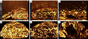
We developed a new method for classifying the images of the contrast-enhanced rectal cancer tumors, which semi-quantitatively categorizes the tumors into 3 types according to the inner texture. The classification criteria were as follows (Figure 1): for class 1 (Figure 1A,1D), the lesion is generally and uniformly enhanced, which means the texture of the tumor is homogeneous; for class 2 (Figure 1B,1E), the lesion is relatively uniformly enhanced, with a small area of hypo-enhancement or nonenhancement, which means the texture of the tumor is relatively inhomogeneous; for class 3 (Figure 1C,1F), the lesion is highly heterogeneously enhanced with a massive area of enhancement deficiency and is eccentric or uneccentric.
The images were classified by 4 colleagues, who were divided into two groups, each consisting of 1 ultrasound physician and 1 medical assistant. First, 500 images were classified by the two groups separately. One month later, they classified the same 500 pictures again. Each image was evaluated by two groups using a blind method. When the categorization of the image by the two groups reached an agreement, this was considered the final result. When no agreement could be reached within or between groups, the image was classified again by the 4 evaluators together. If an agreement was reached, this was considered the final result. If a consensus could still not be reached, the image was excluded from the subsequent analysis.
Computerized method to analyze images
Flowchart of the computer processing steps
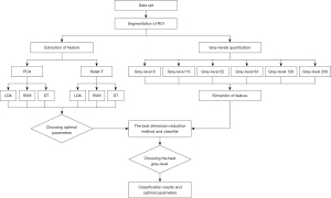
The flowchart of the analysis process is shown in Figure 2. There were 5 main steps: segmentation of ROI, gray level quantization, feature extraction, dimension reduction, and training classifiers one after another.
ROI selection and segmentation
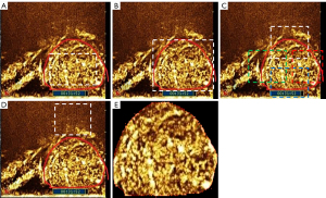
Mainstream ROI selection methods can be categorized as ROIin, ROIout, ROIoverlaps, and ROIposterior (Figure 3) (20). We manually segmented the ROI and proposed the ROI selection based on ROIout with some modifications (Figure 3E). All information outside the tumor boundary was removed. Dimension reduction methods included principal component analysis (PCA) and Relief-F. Classifiers included support vector machines (SVM), decision tree (DT), and linear discriminant analysis (LDA).
Then, 360-dimensional simplified GLCM features were extracted from the ROI. There are redundant and irrelevant features among these features. Texture features underwent dimension reduction and were classified. The best combination was chosen from the 6 combinations of dimension reduction and classifiers. After the dimension reduction method and the classifier were determined, the gray level range of the ROI was determined as one of the six quantization levels. The gray level that performed best in model was selected.
The optimal gray level for reducing noise
The size of GLCM was determined by the gray level of the images (21). The higher the gray level is, the greater the time consumption for computing the GLCM. Gray level is an important factor in the calculation of texture, and the selection of the appropriate gray level can also reduce the classification error rate (22). The effect of noise can be reduced to a certain extent by gray-level quantization (23). In this study, the following uniform quantization strategy was adopted for gray-level quantization:
where I is the original input image, Gmin is the minimum grayscale, Gmax represents the maximum grayscale, K represents the quantization level, and Inew is the processed image.
Extraction of texture features
GLCM is a second-order matrix and is a function of distance and direction. It represents the frequency of occurrence of pixel pairs with gray values y1 and y2. Unser (24) showed that GLCM texture features can be simplified to be directly estimated from the sum and difference histogram, which can replace the large 2D co-occurrence histogram with two 1D histograms and is nearly as accurate for classification. In the study by Haralick et al. (21), among the 14 GLCM features examined, 9 could be directly calculated using the sum and difference histogram, while the remaining 5 could be approximately calculated. The method to extract texture is given in the study by Unser M (24). Altogether, 40 pairs of sum and difference histograms were obtained in the given 10 relative distances and 4 directions. Nine texture features were extracted from each pair of sum and difference histograms, and thus the final number of texture features was 360. The methods to calculate the sum and difference histogram and texture features are given in Appendix 1.
Dimension reduction and classification
In machine learning, dimensionality simply refers to the number of features. To select the features that are helpful for classification, it is necessary to reduce the dimension of the extracted features. Dimension reduction can remove the uncorrelated features to improve the interpretation of the features for the machine learning model. Various methods have been used to reduce dimensionality (25). In the present study, we only compared PCA with Relief-F. After dimension reduction, we aimed to classify rectal CEUS images. The simplified GLCM texture features of the image were used as input, and the output was the class of CEUS image. We used LDA, SVM, and DT to classify the texture features of the image.
Evaluation of the results of the computer classification
Ten-fold cross-validation was used to generate the training set and test set. Ten-fold cross-validation is suitable for small data sets and can yield reliable and stable models. The data were randomly divided into 10 groups. Each subgroup was used as the test set in turn while the remaining 9 groups were used as the training set.
Statistical analysis
Receiver operator characteristic (ROC) analysis was used to evaluate the performance of computer classification. Some diagnostic metrics, including accuracy and area under the curve (AUC), were calculated. All the experiments were conducted in MATLAB 2016a (MathWorks, Natick, MA, USA) and SPSS 23.0 (IBM Corp., Armonk, NY, USA).
Validate phase
Ninety-seven ultrasonograms of contrast-enhanced rectal tumors were collected as validation set from 2018.1 to 2018.6. The inclusion and exclusion criteria were the same as those in the development phase. These images are used to verify the accuracy of the model.
Results
The results of manual classification
The study examined 500 images. The results of manual classification were 121 images for class 1, 172 images for class 2, and 207 images for class 3. The intragroup and intergroup consistency of manual classification was calculated to be 0.95 and 0.92, respectively.
Segmentation
The ROI of all images was successfully segmented, and the results of segmentation were consistent with the manually delineated tumor boundaries. In Figure 1A-1C are the original images of class 1, class 2, and class 3, respectively. Figure 1D-1F shows the results of segmentation. It can be seen from Figure 1D-1F that the information outside the tumor boundary was removed and only the information of the tumor itself was retained.
Feature reduction
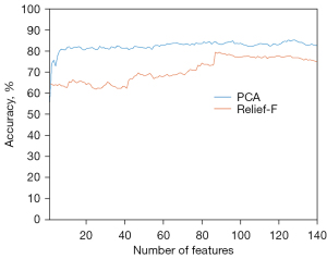
Among the 360 GLCM features used for classification, not all were useful. PCA and Relief-F were first applied to reduce the dimensions of features, which was followed by the application LDA classifiers to distinguish the features. The accuracy of PCA and Relief-F was calculated. PCA had a higher accuracy than did Relief-F. The best accuracies achieved by PCA and by Relief-F were 85.20% (426/500) and 79.40% (397/500), respectively (Figure 4).
Classifiers
The classification accuracies of LDA, SVM, and DT were summarized (Table 1). When the same dimensionality reduction method was used, the accuracy of SVM in image classification is higher than was higher than that of LDA and DT. PCA worked better than did Relief-F on LDA and SVM. However, Relief-F worked better than did PCA on DT. The combination of PCA and SVM achieved the highest accuracy (433/500, 86.60%).
Table 1
| Dimension reduction methods/classifiers | LDA | SVM | DT |
|---|---|---|---|
| PCA | 85.20% | 86.60% | 76.60% |
| Relief-F | 79.40% | 85.80% | 78.20% |
Both PCA and Relief-F are methods to reduce dimension. LDA, SVM and DT are three classifiers to distinguish CEUS images. PCA, principal component analysis; LDA, linear discriminant analysis; SVM, support vector machines; DT, decision tree; CEUS, contrast-enhanced ultrasound.
Influence of gray-level quantization
Results of different gray level quantization are shown in Figure 5. The first column in Figure 5A is the unprocessed image, and the second to seventh columns are the results of quantizing the grayscale of the image to 8, 16, 32, 64, 128, and 256. As shown in Figure 5, pixels with similar gray values were merged by quantization.

The accuracy of SVM at different gray-level quantization is shown in Figure 6. Each line chart shows the change of accuracy as the number of features. The line chart of different colors represents the experimental results of different gray levels. All curves fluctuated upward and then stabilized. After selection for the appropriate number of features, the accuracy of all 6 experiments exceeded 80%. When the same number of features was selected for the experiment, in most cases, the classification accuracy of gray level 32 was higher than that of any other gray level. Table 2 shows the best classification accuracy (mean ± standard deviation) achieved by different gray levels and the number of features corresponding to the best accuracy. The best accuracy of gray level 32 was 87.80% (439/500), which was higher than the other gray levels. This suggests that the gray level has a certain degree of influence on the classification results.
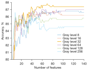
Table 2
| Gray level | 8 | 16 | 32 | 64 | 128 | 256 |
|---|---|---|---|---|---|---|
| Number of features | 90 | 61 | 69 | 63 | 42 | 8 |
| Accuracy (%) | 86.80±4.40 | 86.80±4.54 | 87.80±4.47 | 87.00±3.43 | 86.80±3.29 | 86.60±4.12 |
The best classification accuracy (mean ± standard deviation) achieved by different gray levels and the number of features corresponding to the best accuracy.
Comparison of manual and computer classification results
We set optimal parameters and classified the images. PCA was used for feature selection, and 69 features were selected. SVM was implemented to distinguish rectal CEUS images. Table 3 shows the comparison between the result of manual classification and that of computer classification. A total of 121 images were manually classified into class 1, and 121 were classified into class 1 by computer; 172 images were classified into class 2 manually, and 181 images were classified into class 2 by computer; 207 images were classified into class 3 manually, and 198 images classified into class 3 by computer. There were 439 images with consistent classification results between both methods. The number of cases that the computer classified from class 1 erroneously into class 3 was zero. The number of cases that the computer classified from class 3 erroneously into class 1 was zero. The main errors were that the computer classified the images of class 1 and class 3 into class 2 or classified the images of class 2 into class 1 or class 3. The ROC curve is shown in the supplementary materials (Figure S1). The AUC of class 1, 2, and 3 was 0.97, 0.93, and 0.98, respectively.
Table 3
| Manual classification | Computer classification | Total | ||
|---|---|---|---|---|
| 1 | 2 | 3 | ||
| 1 | 104 | 17 | 0 | 121 |
| 2 | 17 | 146 | 9 | 172 |
| 3 | 0 | 18 | 189 | 207 |
| Total | 121 | 181 | 198 | 500 |
Validation phase
Data collection and classification
A total of 97 ultrasonograms of contrast-enhanced rectal tumors were included. The images were divided into 3 classes according to the abovementioned standards. Computing methods were used to simulate manual classification. The performance of manual and computer classification was evaluated and compared.
Accuracy of computer classification in the validation cohort
The ability of the computer to predict the tumor inhomogeneity in rectal cancer CEUS images was evaluated in the validation cohort. SVM and gray level 32 were used to distinguish rectal CEUS images. Table 4 shows the result of the comparison between manual classification and that of computer classification. A total of 59 images had consistent classification results by both methods (60.82%). The main errors were that the computer classified the images of class 1 and class 3 into class 2 or classified the images of class 2 into class 1 or class 3. The ROC curve is shown in the supplementary materials (Figure S2). The AUC of class 1, 2, and 3 was 0.76, 0.41, and 0.48, respectively.
Table 4
| Manual classification | Computer classification | Total | ||
|---|---|---|---|---|
| 1 | 2 | 3 | ||
| 1 | 23 | 12 | 1 | 36 |
| 2 | 5 | 13 | 10 | 28 |
| 3 | 0 | 10 | 23 | 33 |
| Total | 28 | 35 | 34 | 97 |
Discussion
The inhomogeneity of contrast-enhanced rectal cancers in ultrasonograms can provide reference information with the details of rectal tumors vasculature, but the judgment of inhomogeneity depends on the training, experience, and expertise of the radiologists. Computer technology can assist doctors in routine diagnostic work to obtain more accurate, objective, and reproducible results.
Common applications of computer technology in medical imaging include automatic measurement, automatic detection and segmentation of tissue, and classification of benign and malignant tissues. In recent years, artificial intelligence, especially deep learning, has made the classification task of benign and malignant tissues increasingly convenient and accurate. As a branch of artificial intelligence, traditional machine learning involves data cleaning, feature extraction, dimensionality reduction, and training the model. Traditional machine learning is well supported by theoretical foundations; therefore, it is easier for researchers to design a model and adjust the hyperparameters. Feature extraction is the process of extracting image information by computer. As a kind of feature extraction, texture feature is widely used in medical image analysis. Some studies use the texture feature to classify lesions and injuries or distinguish between benign and malignant tumors, indicating that texture analysis is an effective method for analyzing ultrasonograms (26-30). In the present study, we focused on the inhomogeneity of contrast-enhanced rectal cancers in ultrasonograms and found that this was closely related to the distribution of microvessels. Therefore, we classified the inhomogeneity of contrast-enhanced rectal cancers in ultrasonograms by using texture information and machine learning. Results showed that the computer methods were competent for classifying the inhomogeneity of contrast-enhanced rectal cancers inside ultrasonograms.
The ROI selected, the relative direction and distance of features, and the gray level of the image can influence classification results produced by models. The most commonly used method of ROI selection is ROIout, through which the texture information regarding the internal and external parts of the lesion can be extracted (20,27,30). The advantage of the ROIout method is that the information concerning the lesion’s surroundings can be obtained. However, if this secondary information has no relevance to the lesion, it becomes a kind of interference. Our study only focused on the inhomogeneity of contrast-enhanced rectal cancers in ultrasonograms; therefore, any information concerning the lesion’s surroundings was excluded. We used a mask to mark the lesion itself and then calculated only the texture information of the lesion area. Any information regarding outside the lesions area that could be interference was therefore discarded.
The texture information is related to the direction and distance of pixels. Therefore, the choice of GLCM direction and distance becomes particularly important. A few studies empirically chose the direction and distance of the texture, with only 4 directions and 1 distance being considered (18,20). Empirically selecting the texture distance and direction of GLCM may lead to inadequate texture information being extracted. We calculated texture from 10 distances and 4 directions to enrich the texture information. A total of 360 texture features were extracted, and irrelevant information was shrunk by dimension reduction. The PCA algorithm achieved higher accuracy than did the Relief-F algorithm. While texture features totaled 360, the final number of features for classification was only 69. This indicated that the 69 features contained enough information to classify the inhomogeneity of rectal CEUS. The 3 different classifiers of LDA, SVM, and DT were also compared, among which SVM performed the best.
In addition, we studied the influence of gray quantization on the classification results. We found that classification accuracy was improved by gray-level quantization and that pixels with similar values were merged by gray-level quantization, which reduced noise to some extent. If the gray level was too high or too low, the accuracy of the model will decrease. By comparing the experimental results of different gray-level quantization, we found that gray level 32 produced the highest classification accuracy, and was hence the best choice.
The degree of inhomogeneity of class 2, which was between class 1 and class 3, therefore is more challenging for radiologists to distinguish. This difficulty was also encountered in the computer classification: the AUC of class 2 was lower than that of class 1 and class 3.
Despite these findings, the present study had 3 major limitations. First, our results may be biased because data in this study were collected from the same type of equipment, without considering the impact of different devices on image quality. Images from different devices should be considered for analysis in the future. Second, our data for analysis were static and not dynamic because we only focused on the images at peak moments and did not consider the dynamic change during the whole period of contrast. Future research should examine the impact of the changing process of contrast enhancement by analyzing the features of CEUS images in a time series. Finally, we did not conduct any comparative studies between clinical and pathological results, and thus further research in this vein is still needed.
Acknowledgments
The authors thank Zhang Qiong and Jing Jigang for supporting this work as part of HZ, PhD’s work. We also thank Liu Xueting for her statistical comments during the review process.
Funding: The study was supported by
Footnote
Reporting Checklist: The authors have completed the STARD reporting checklist. Available at https://tcr.amegroups.com/article/view/10.21037/tcr-21-2362/rc
Data Sharing Statement: Available at https://tcr.amegroups.com/article/view/10.21037/tcr-21-2362/dss
Conflicts of Interest: All authors have completed the ICMJE uniform disclosure form (available at https://tcr.amegroups.com/article/view/10.21037/tcr-21-2362/coif). The authors have no conflicts of interest to declare.
Ethical Statement: The authors are accountable for all aspects of the work in ensuring that questions related to the accuracy or integrity of any part of the work are appropriately investigated and resolved. The study was conducted in accordance with the Declaration of Helsinki (as revised in 2013). This retrospective study was additionally part of a clinical trial. The corresponding trial (registration no. ChiCTR-RNC-10000932) was approved and supervised by West China Hospital, Sichuan University’s Institutional Review Board. Individual consent for this retrospective study was waived.
Open Access Statement: This is an Open Access article distributed in accordance with the Creative Commons Attribution-NonCommercial-NoDerivs 4.0 International License (CC BY-NC-ND 4.0), which permits the non-commercial replication and distribution of the article with the strict proviso that no changes or edits are made and the original work is properly cited (including links to both the formal publication through the relevant DOI and the license). See: https://creativecommons.org/licenses/by-nc-nd/4.0/.
References
- Chen W, Zheng R, Baade PD, et al. Cancer statistics in China, 2015. CA Cancer J Clin 2016;66:115-32. [Crossref] [PubMed]
- Wang XS. Epidemiological characteristics and prevention and control strategies of colorectal cancer in China and American. Chinese Journal of Colorectal Diseases 2019;8:1-5.
- Cârțână ET, Gheonea DI, Săftoiu A. Advances in endoscopic ultrasound imaging of colorectal diseases. World J Gastroenterol 2016;22:1756-66. [Crossref] [PubMed]
- Al-Sukhni E, Milot L, Fruitman M, et al. Diagnostic accuracy of MRI for assessment of T category, lymph node metastases, and circumferential resection margin involvement in patients with rectal cancer: a systematic review and meta-analysis. Ann Surg Oncol 2012;19:2212-23. [Crossref] [PubMed]
- Phang PT, Gollub MJ, Loh BD, et al. Accuracy of endorectal ultrasound for measurement of the closest predicted radial mesorectal margin for rectal cancer. Dis Colon Rectum 2012;55:59-64. [Crossref] [PubMed]
- Anderson H, Price P, Blomley M, et al. Measuring changes in human tumour vasculature in response to therapy using functional imaging techniques. Br J Cancer 2001;85:1085-93. [Crossref] [PubMed]
- Bensaad K, Harris AL. Hypoxia and metabolism in cancer. Adv Exp Med Biol 2014;772:1-39. [Crossref] [PubMed]
- Loria F, Loria G, Basile S, et al. Role of contrast-enhanced ultrasound in the evaluation of vascularization of hepatocellular carcinoma. Hepatoma Research 2016;2:316-22. [Crossref]
- Wang Y, Li L, Wang YX, et al. Time-intensity curve parameters in rectal cancer measured using endorectal ultrasonography with sterile coupling gels filling the rectum: correlations with tumor angiogenesis and clinicopathological features. Biomed Res Int 2014;2014:587806. [Crossref] [PubMed]
- Valentino M, De Matteis M, Casadio Baleni M, et al. Contrast-enhanced US of the prostate with time/intensity curves: Preliminary results. J Ultrasound 2008;11:8-11. [Crossref] [PubMed]
- Giangregorio F, Bertone A, Fanigliulo L, et al. Predictive value of time-intensity curves obtained with contrast-enhanced ultrasonography (CEUS) in the follow-up of 30 patients with Crohn's disease. J Ultrasound 2009;12:151-9. [Crossref] [PubMed]
- Krizhevsky A, Sutskever I, Hinton GE. ImageNet classification with deep convolutional neural networks. Communications of the ACM 2017;60:84-90. [Crossref]
- Simonyan K, Zisserman A. Very deep convolutional networks for large-scale image recognition. arXiv 2014. arXiv:1409.1556.
- Attia MW, Abou-Chadi FEZ, Moustafa HED, et al. Classification of ultrasound kidney images using PCA and neural networks. International Journal of Advanced Computer Science and Applications 2015;6:53-7.
- Mohammed MA, Al-Khateeb B, Rashid AN, et al. Neural network and multi-fractal dimension features for breast cancer classification from ultrasound images. Computers & Electrical Engineering 2018;70:871-82. [Crossref]
- Foster KR, Koprowski R, Skufca JD. Machine learning, medical diagnosis, and biomedical engineering research - commentary. Biomed Eng Online 2014;13:94. [Crossref] [PubMed]
- Liu T, Yang X, Curran W, et al. TU‐F‐12A‐09: GLCM Texture Analysis for Normal-Tissue Toxicity: A Prospective Ultrasound Study of Acute Toxicity in Breast-Cancer Radiotherapy. Medical Physics 2014;41:482. [Crossref]
- Sharma K, Virmani J. A decision support system for classification of normal and medical renal disease using ultrasound images: a decision support system for medical renal diseases. International Journal of Ambient Computing and Intelligence 2017;8:52-69. (IJACI). [Crossref]
- Shrimali V, Anand RS, Kumar V. Current trends in segmentation of medical ultrasound B-mode images: a review. IETE Technical Review 2009;26:8-17. [Crossref]
- Jeon JH, Choi JY, Lee S, et al. Multiple ROI selection based focal liver lesion classification in ultrasound images. Expert Syst Appl 2013;40:450-7. [Crossref]
- Haralick RM, Shanmugam K, Dinstein IH. Textural features for image classification. IEEE Trans Syst Man Cybern 1973;SMC-3:610-21. [Crossref]
- Soh LK, Tsatsoulis C. Texture analysis of SAR sea ice imagery using gray level co-occurrence matrices. IEEE Trans Geosci Remote Sens 1999;37:780-95. [Crossref]
- Gomez W, Pereira WC, Infantosi AF. Analysis of co-occurrence texture statistics as a function of gray-level quantization for classifying breast ultrasound. IEEE Trans Med Imaging 2012;31:1889-99. [Crossref] [PubMed]
- Unser M. Sum and difference histograms for texture classification. IEEE Trans Pattern Anal Mach Intell 1986;8:118-25. [Crossref] [PubMed]
- Roffo G, Melzi S, Cristani M. Infinite feature selection. In: Proceedings of the IEEE International Conference on Computer Vision. 2015:4202-10.
- Lee S, Jo IA, Kim KW, et al. Enhanced classification of focal hepatic lesions in ultrasound images using novel texture features. In: 2011 18th IEEE International Conference on Image Processing. IEEE, 2011:2025-8.
- Xian G. An identification method of malignant and benign liver tumors from ultrasonography based on GLCM texture features and fuzzy SVM. Expert Syst Appl 2010;37:6737-41. [Crossref]
- Rahmawaty M, Nugroho HA, Triyani Y, et al. Classification of breast ultrasound images based on texture analysis. In: 2016 1st International Conference on Biomedical Engineering (IBIOMED). IEEE, 2016:1-6.
- Abdel-Nasser M, Melendez J, Moreno A, et al. Breast tumor classification in ultrasound images using texture analysis and super-resolution methods. Eng Appl Artif Intell 2017;59:84-92. [Crossref]
- Nugroho HA, Rahmawaty M, Triyani Y, et al. Texture analysis for classification of thyroid ultrasound images. In: 2016 International Electronics Symposium (IES). IEEE, 2016:476-80.
(English Language Editors: C. Mullens and J. Gray)


